(this post originated in The second edition of my newsletter)

The goal of this post is to walk everyone through how an LSM Tree works. I'll do my best to not wander off into philosophical questions and trying to reason about "why" it is the way it is, and focus more on "so what". I promise that i'll get to the rambling at some point though :D

Table of Contents

1. What is an LSM Tree?
2. Immutability as an operating principle
3. The LSM Tree Architecture
4. The Write Path
5. The Read Path
6. Formalizing our understanding of performance
7. Why is too many files bad, and how do we fix it?
8. Compaction

What is an LSM Tree?

An LSM Tree is a disk-based data structure that's used to store key-value pairs on disk. A disk-backed KV (Key-Value) Store is a foundational building block for many applications, so doing this well is important. The main focus of a key-value store is persistence, so it's obvious that the disk, and files, are involved somewhere - we're going to see how and where.

Simply put, the job of the LSM Tree (and most other storage structures) is to obey the following interface, while ensuring that the data you've added or modified stays as it is between crashes and restarts.

LSMTree {
	fn Upsert(String key, String value)
	fn Delete(String key)
	fn Get(String key) -> Option<String>
}

That's the functional requirement. Non-functional requirements are varied and many, including, but not limited to:

1. Take as less disk space as possible
2. Make the reads fast
3. Make the writes fast
4. Make everything fast (Jury's out on whether or not this is a functional requirement, but for the sake of this post, let's assume it isn't)

Compared to other, more conventional data structures that also do the same thing (for example, B-Trees), the LSM Tree really shines when used with write-heavy workloads. An important distinction is that LSM Trees do not update data in-place - data, once written to disk, is guaranteed to be immutable, and will only ever be rewritten into a new file at some point. This lets LSM Trees have much cheaper writes than other data structures that perform in-place modifications to existing data files.

Let's first explore what out-of-place updates are, and then we'll investigate how the core data structure actually works.

An Immutable Database? What the hell is that?

The fundamental question remains - how do you overwrite or delete data if the on-disk data structure is immutable? The simplest answer is - to create another on-disk data structure that represents this, and ensure you read all data on disk in the order of newest to oldest.

To motivate this idea, let's take an example of a simple JSON file (data.1) where we have three key-value pairs. The filename is important as it helps us gain an understanding of the order in which the files were written.

// data.1
{
	"backstreet boys": "show me the meaning of being lonely",
	"metallica": "one",
	"charanjit singh": "kalavati",
}

Let us say that we wish update the value of the key "metallica" to "for whom the bell tolls" under the specific constraint that we cannot modify the file itself which has the key stored in it.

To show that data has been modified, if I can guarantee that data.(x+1) is always read before data.(x) where x + 1 > x, then I can "modify" the data present by writing data.(x+1) as follows:

// data.2
{
	"metallica": "for whom the bell tolls"
}

Consider our read algorithm to be as follows, essentially enforcing the principles we mentioned earlier:

read(key):
	for file in files.sort(newest_to_oldest):
		for kvpair in file:
			if kvpair.key == key:
				return (true, kvpair.value)
	return (false, "")

In this way, we can guarantee that our reader will always first see the latest value of the key, hence performing a "modification".

Now, you might ask - this works for overwrites; but how does one delete a record? The way we do this is that we frame our deletes as overwrites. If I wish to delete the key "backstreet boys", all I need to do is create a new data file:

// data.3
{
	"backstreet boys": DELETED
}

This is known as a "tombstone". Our reader is then modified to be as follows:

read(key):
	for file in files.sort(newest_to_oldest):
		for kvpair in file:
			if kvpair.key == key:
				if kvpair.value == TOMBSTONE:
					return (false, value)
				return (true, value)
	return (false, "")

Yay! We now have an immutable database. Now, you may be wondering: if all we ever do is write new files, even if data is deleted, how do we avoid making the disk full? Hold on to that question, and let's explore how an LSM Tree actually works.

What makes an LSM Tree?

A record is a pair of strings/bytes, usually both key and value. We can consider a tombstone/deletion marker to be some type of string/byte stream as well, recognized throughout the LSM Tree. We can consider the LSM Tree to be a collection of records, such that you perform CRUD operations via the key. Hence, the atomic unit of data in this LSM Tree is the record.

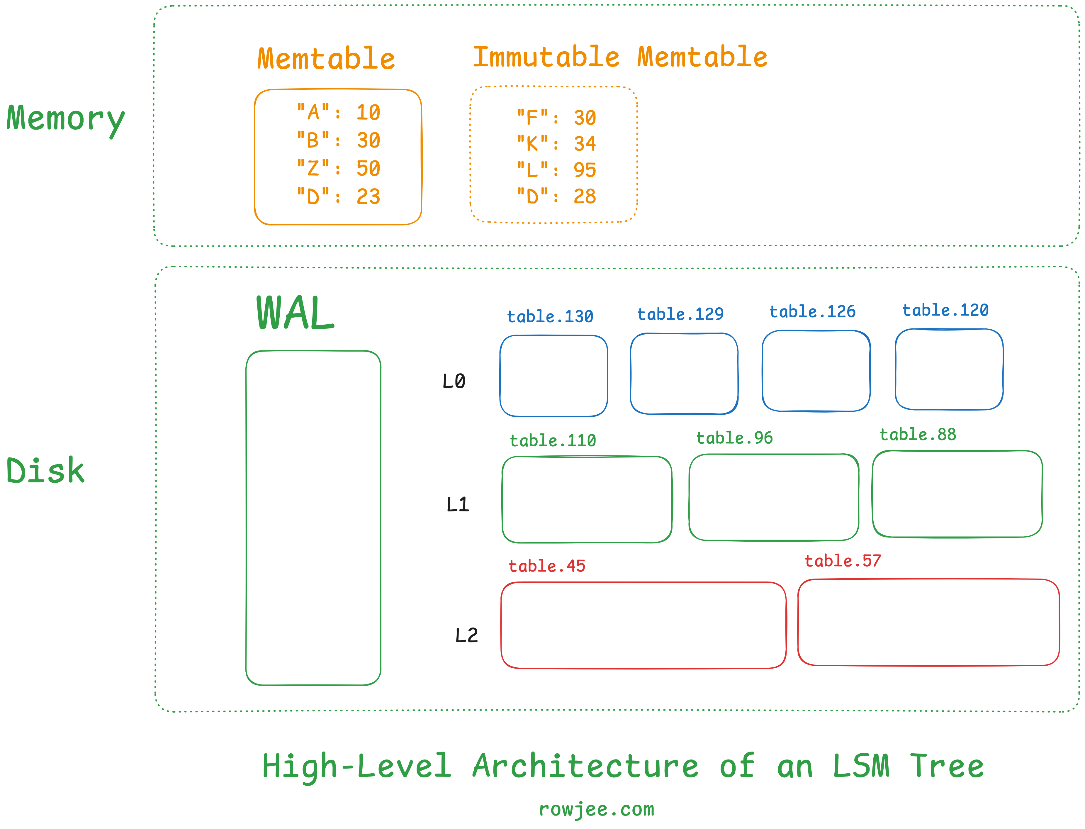
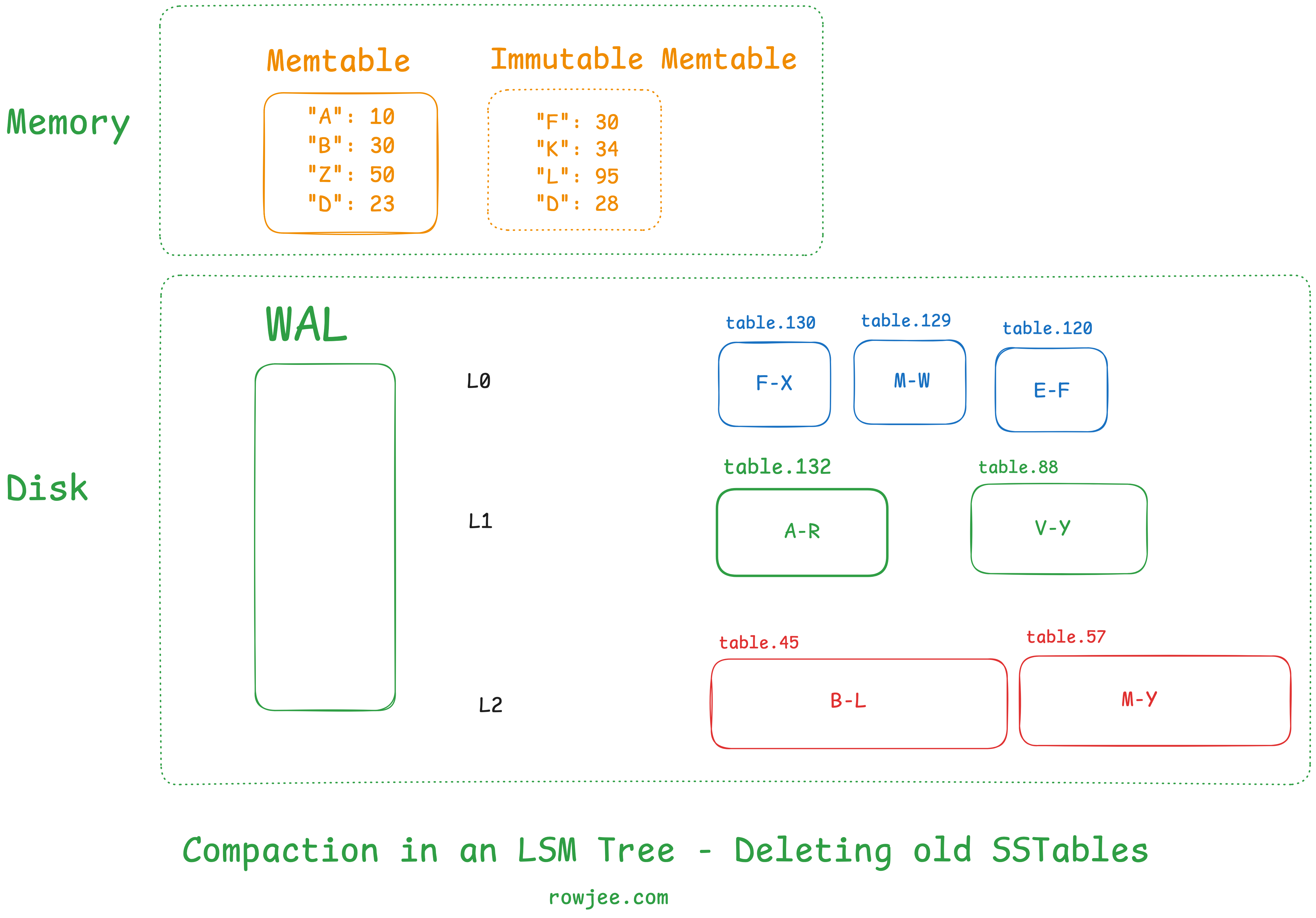
The LSM Tree usually has three components.

Memtable: This is the in-memory component of the LSM Tree. It's usually a fixed size, and all records end up here first, ensuring faster writes. It's usually a hashmap-type data structure that lets us access data via a key-value interface.

Write-Ahead Log (WAL): this disk-based component ensures that we don't encounter data loss if some records are only in the memtable and haven't made it to disk yet. All records are written to the WAL first, and then to the memtable, to ensure that the records have been persisted to disk - this ensures that we're able to recover memtable data if we crash without writing the memtable to disk. We won't be exploring this too much in this post, but it's important to know why it exists.

SSTable files: This is the largest component of the LSM Tree. When a memtable is full, it is "flushed" onto disk, to create one SSTable file. Each file contains a set of records stored in a sorted manner.

this isn't a component, but an important concept nonetheless - Levels: LSM Trees usually store these SSTable files in levels. There are usually five levels, and each level has a cap on the maximum size of an SSTable that can be present inside the levels. There's often a strategy to how we organize the levels themselves, and what heuristics let us keep data in one level vs move it to the other; For now, we can assume that the higher levels have smaller files, fresher data, and that the lower levels have larger files with older, staler data.

Writing some data to an LSM Tree

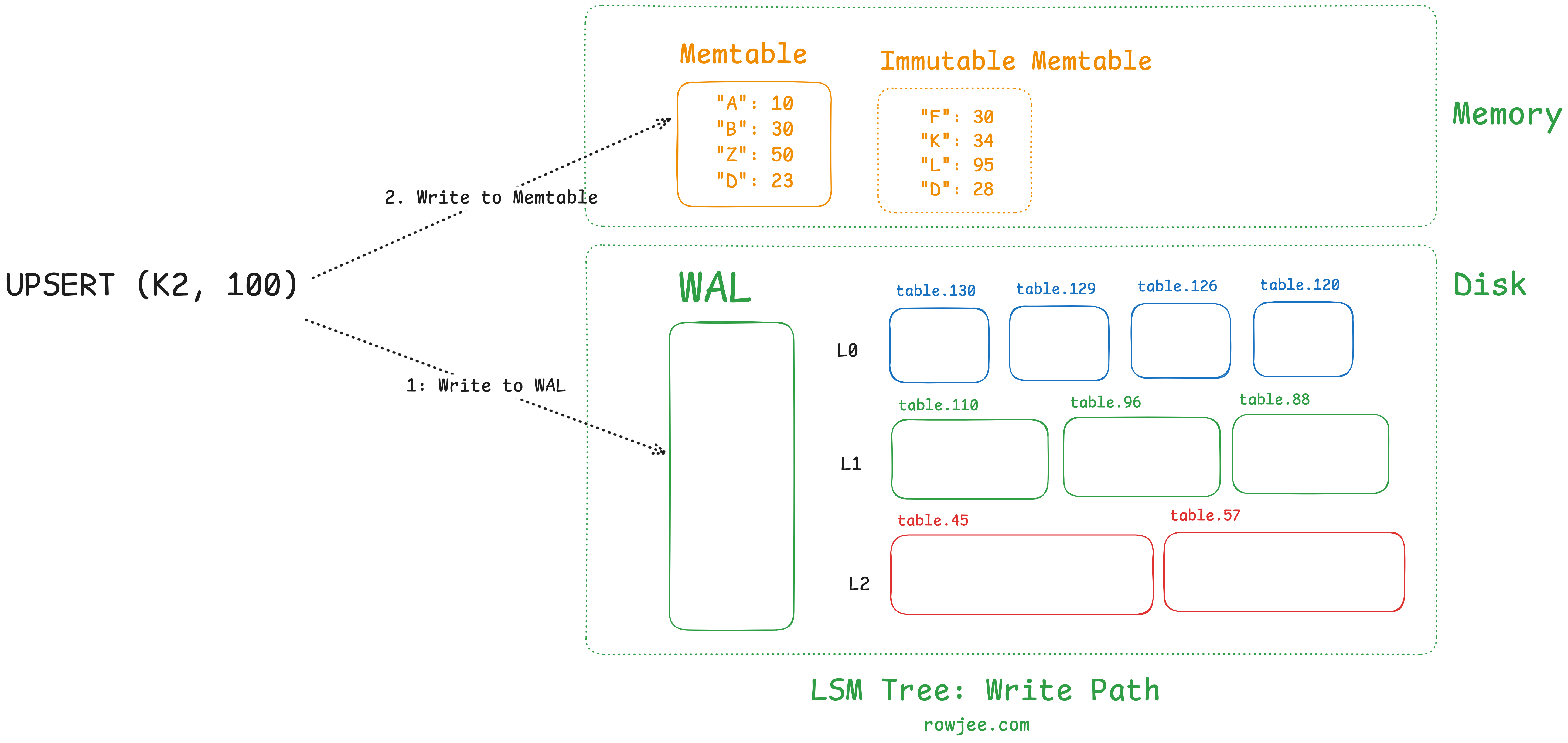
write(key, value)
	write to WAL
	write to memtable
	if memtable is full, write it to disk as an SSTable

Given that the memtable is in-memory, but we still need to offer durability as a guarantee, we will make use of a write-ahead log where all data is persisted to disk by default, and only once it persists in the WAL will we write it to the memtable. This ensures that if the machine crashes after the write completes to the memtable, but isn't present on disk, we do not lose our data.

Flushing Data to disk

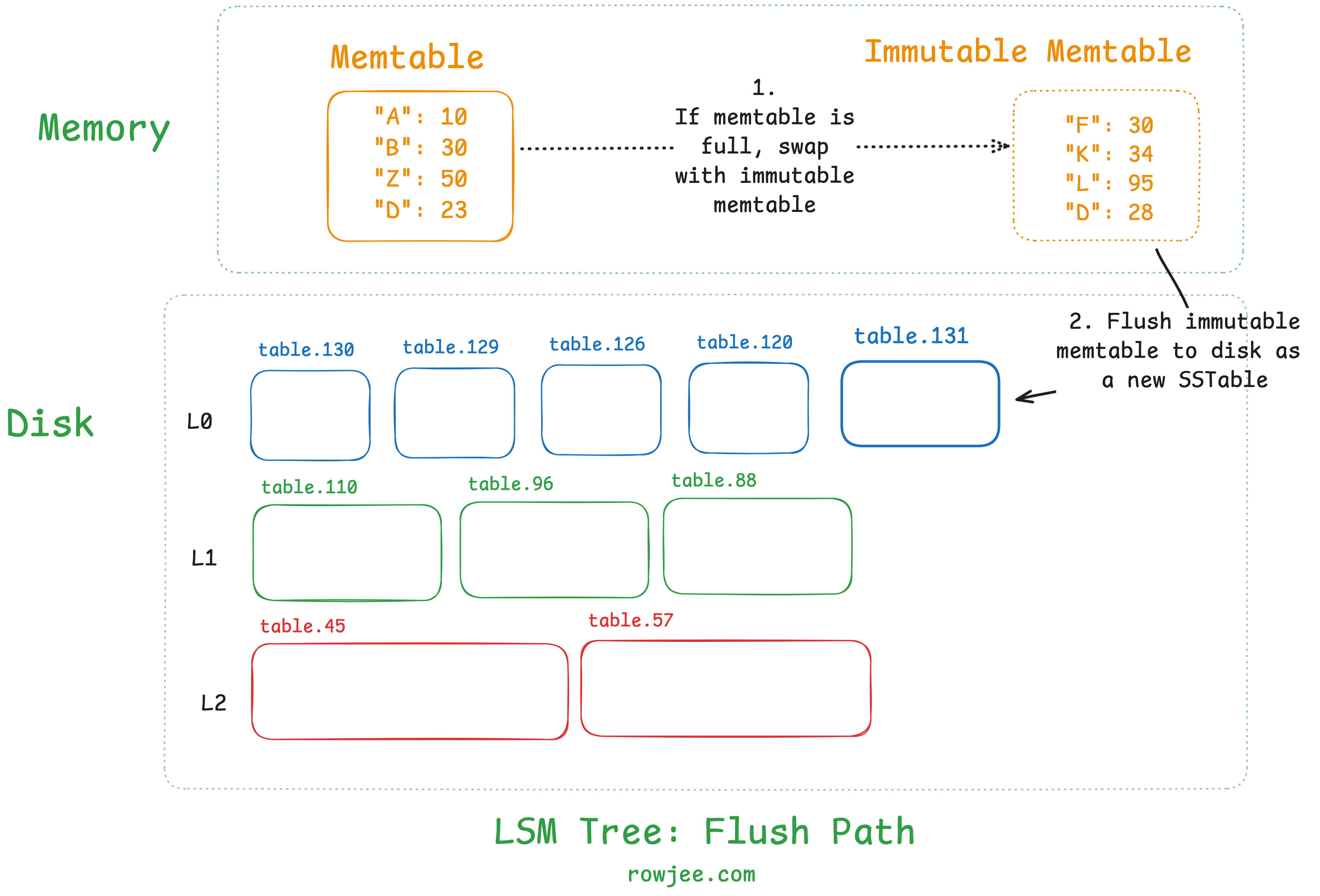
We know that we don't have infinite memory available! Once the memtable goes beyond a defined capacity (either in terms of number of records or in terms of size), the memtable is flushed to disk, as an SSTable. This frees up the memtable to accept new writes, and ensures that our data is reliably persisted to storage.

Most implementations will usually have a second immutable memtable, which is present as a standby; this is because flushing is an operation that involves a disk IO, which, in computer time, can be pretty slow. If we block the memtable from accepting any writes during the flush, it'll be a performance penalty that we don't really want to pay - hence, flushing allows us to swap the active memtable out, replace it with an empty one (thus making the full memtable immutable), and operate on the immutable memtable.

For now, let's assume that we do nothing apart from flushing our memtable into a new SSTable. This means that every time we fill our memetable's memory quota, we will create a new file on disk. This also means that our disk size will grow in a rate proportional to the write rate.

All memtables are flushed into Level 0 of the LSM Tree, without further organization.

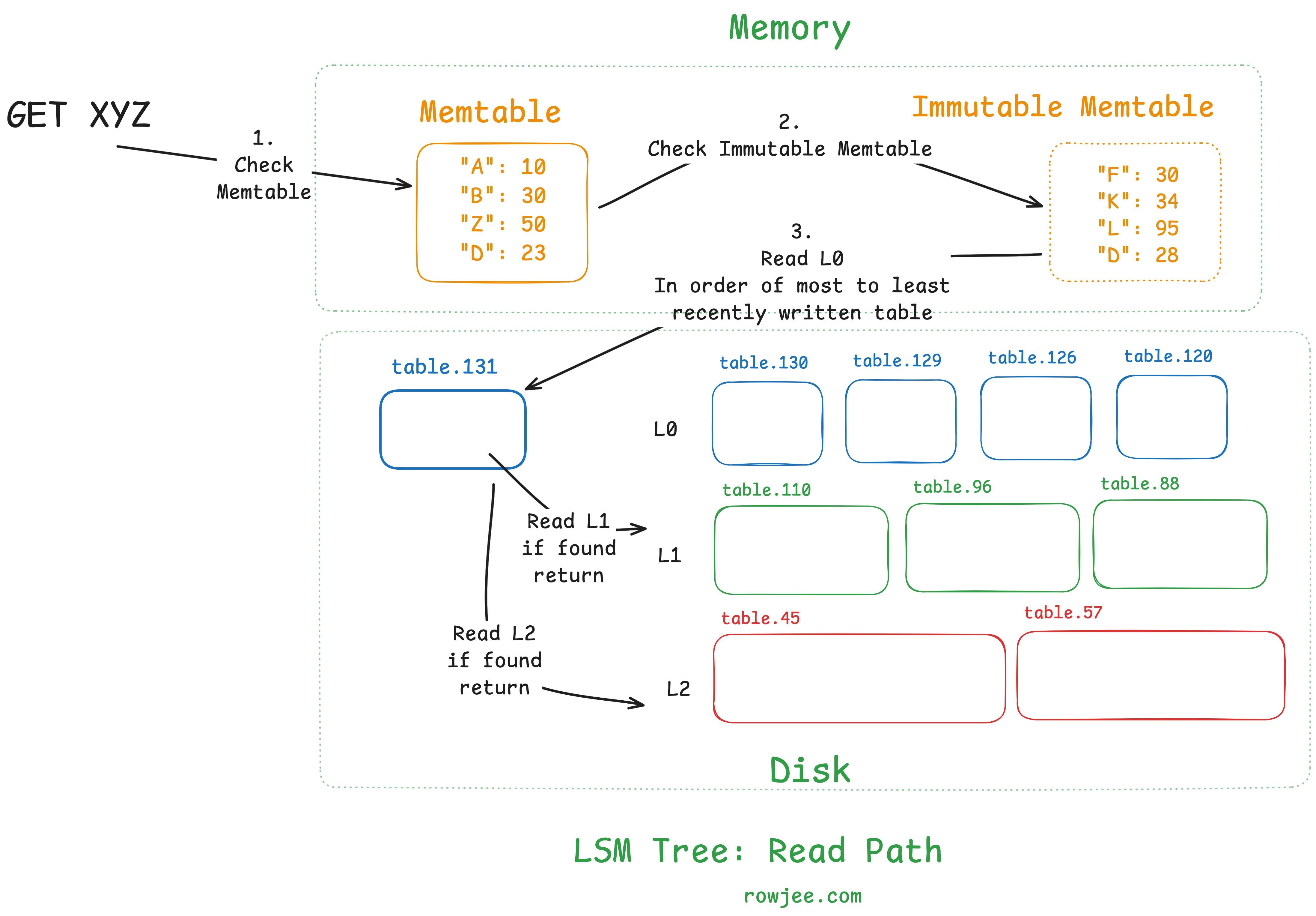
Reading some data from an LSM Tree

search_table(table, key)
	for record in table:
		if key == record.key:
			return found
	return not found

read(key):
	read the memtable
	if found, return
	for level in levels:
		for table in level.sort_by_recent():
			search_table(table, key)
	return "not found"

Let us first understand that to read some data, we need to know where it is. This is the majority of the problem; as data structure designers, we need to ensure that all keys are found (or if not found, confirmed as such) as quickly as possible. Once we know where the data is, reading the disk block is a relatively fixed-time operation.

To find a key, we first search both memtables. If the key was written fairly recently, we maximize our chances of a very cheap read, as we perform no disk IO for this read.

This approach does introduce some problems. Since we don't really maintain any other index, for every key we search, we need to go through every SSTable file. Relatively speaking, opening a file and reading from it is an expensive operation; We would ideally like to minimize this as much as possible. So we need to figure out some way to make reads cheaper, and to avoid opening a large number of files for each read.

To do this, an invariant we maintain is that all levels of the LSM Tree (apart from Level 0) maintain SSTables that comprise only of non-overlapping key ranges. This means that when we look at a particular level, a key can belong only to one SSTable in that level - this is to ensure that we have at most one file to search through in each level of the tree.

Once we do this, our algorithm looks something like this:

search_table(table, key)
	for record in table:
		if key == record.key:
			return found
	return not found

read(key):
	read the memtable
	if found, return
	for level in levels:
		if level == level0:
			for table in level.sort_by_recent():
				search_table(table, key)
		else:
			table = find_table() # there can only be one
			search_table(table, key)
	return "not found"

Formalizing our understanding of performance

let's look at two new terms that'll help us understand how to reason about performance in storage systems. We can use them as a sort of Big-O notation to reason about which storage algorithms are efficient, and which aren't.

read amplification: the ratio of bytes read to read a value, to the size of the value
write amplification: the ratio of bytes written to write a value, to the size of the value
space amplification: "Space-amp is the ratio of the size of the database to the size of the data in the database"¹

In a B-Tree, write amplification is high, because every write causes you to potentially split the parent node pages into new ones, which you will also have to write to disk. Conversely, the read amplification is pretty low, because you only need to read log_2(branch_factor) disk pages due to the nature of the B-Tree.

Let's go back to our case of the LSM Tree so far; we don't do anything to the SSTable files once they're written as a part of the flush process. This means that if we have a key that we want to look up, we're going to have to basically read through most, if not all, of the files present - this causes massive read amplification. This is also harmful from a performance point of view, because what could have been 1 I/O syscall with an in-memory index, is now a potentially unbounded number.

Given that the LSM Tree we know in this article so far, is optimized for low write amplification - a near perfect factor of 1, because we write all data to a new file regardless - we now need to figure out how to reduce the read amplification of the LSM Tree to make sure it's reasonably performant.

Why is too many files bad, and how can we fix it?

As of right now, we already know that we have a pretty fast write path; data hits memory first and stays in memory until the memtable is full, beyond which point we need to flush the data to disk. Measured by I/O, these writes are very, very cheap (1 I/O), but in the grand scheme of things, not free - we will now incur a cost that we need to pay on every read.

The situation we are at so far is as follows:

1. If we need to read the disk, we need to read all SSTables as they all have overlapping ranges, so we can't really say which specific table has data. It could be present in multiple tables. This will incur high read amplification.
2. Our SSTables will each be as small as the memtable size quota, which means that we'll need to be doing a large number of random disk IOs to read all the SSTables. This is the exact problem that manifests in B-Trees that we are trying to avoid (Modern day SSDs handle this much better, but we'll get to that in another post).
3. We are never reclaiming data from the disk; no matter how many times a record is overwritten or deleted, the original record still exists on disk. This is wasteful.

Given the problems, we need to implement some kind of solution that

1. Keeps the disk size from growing at an unbounded rate
2. Limits the number of small files present by grouping more data on disk together, allowing for a larger file to be created and accessed with fewer IOs
3. Maintains the invariant of non-overlapping ranges

Let's go back to the previous example we have.

// data.1
{
	"backstreet boys": "show me the meaning of being lonely",
	"metallica": "one",
	"charanjit singh": "kalavati",
}
// data.2
{
	"metallica": "for whom the bell tolls"
}
// data.3
{
	"backstreet boys": DELETED
}
// let's add some more music here
// data.4
{
	"moblack": "yamore",
	"AC/DC": "thunderstruck",
	"gorillaz": "feel good inc",
}
// data.5
{
	"charanjit singh": "raag bhairav",
	"death cab for cutie": "i'll follow you into the dark",
	"daft punk": "instant crush"
}

We can clearly see that we're overwriting some data - remember, we need only keep the latest value - and we're deleting some data too.

What if we were able to pre-compute the outcome of a read (per the algorithm we described) for this set of files? If we can ensure that the read function works the same on two different representations of data, while one takes lesser space, and is correct (in that we get the same values we stored per key, for every key), would it not be better to perform said computation in the background?

By doing this, we have solved a bunch of the problems we have, by:

1. Converting many small files into one large file
2. Removing overwritten/deleted data
3. Can also move the data into clear non-overlapping ranges

This is the process known as compaction, which is a background task that works to maintain the disk space used by frequently merging SSTable files such that disk usage is kept at a reasonable level, while lookup latency is also managed by ensuring that we don't have too many small files to open.

Compaction: Merging multiple SSTable files into one

So, let's start with the following motivation:

What do I need to do to maintain the same data, but with lesser space?

// data.1
{
	"backstreet boys": "show me the meaning of being lonely",
	"metallica": "one",
	"charanjit singh": "kalavati",
}
// data.2
{
	"metallica": "for whom the bell tolls"
}
// data.3
{
	"backstreet boys": DELETED
}
// let's add some more music here
// data.4
{
	"moblack": "yamore",
	"AC/DC": "thunderstruck",
	"gorillaz": "feel good inc",
}
// data.5
{
	"charanjit singh": "raag bhairav",
	"death cab for cutie": "i'll follow you into the dark",
	"daft punk": "instant crush"
}

A good place to start is to know that we need to maintain key ordering even in the final table, so let's start by ordering all the data (across files) by key; Since the order of writing (AKA the SSTable ID) is important, we'll keep that around, too.

[
	{"tableID": 1, "data": {"backstreet boys": "show me the meaning of being lonely"}},
	{"tableID": 1, "data": {"metallica": "one"}},
	{"tableID": 1, "data": {"charanjit singh": "kalavati"}},
	{"tableID": 2, "data": {"metallica": "for whom the bell tolls"}},
	{"tableID": 3, "data": {"backstreet boys": DELETED}},
	{"tableID": 4, "data": {"moblack": "yamore"}},
	{"tableID": 4, "data": {"AC/DC": "thunderstruck"}},
	{"tableID": 4, "data": {"gorillaz": "feel good inc"}},
	{"tableID": 5, "data": {"charanjit singh": "raag bhairav"}},
	{"tableID": 5, "data": {"death cab for cutie": "i'll follow you into the dark"}},
	{"tableID": 5, "data": {"daft punk": "instant crush"}}
]

First ordering by key:

[
	{"tableID": 4, "data": {"AC/DC": "thunderstruck"}},
	{"tableID": 1, "data": {"backstreet boys": "show me the meaning of being lonely"}},
	{"tableID": 3, "data": {"backstreet boys": DELETED}},
	{"tableID": 1, "data": {"charanjit singh": "kalavati"}},
	{"tableID": 5, "data": {"charanjit singh": "raag bhairav"}},
	{"tableID": 5, "data": {"daft punk": "instant crush"}},
	{"tableID": 5, "data": {"death cab for cutie": "i'll follow you into the dark"}},
	{"tableID": 4, "data": {"gorillaz": "feel good inc"}},
	{"tableID": 1, "data": {"metallica": "one"}},
	{"tableID": 2, "data": {"metallica": "for whom the bell tolls"}},
	{"tableID": 4, "data": {"moblack": "yamore"}},
]

Then, ordering from most recently written to least:

[
	{"tableID": 4, "data": {"AC/DC": "thunderstruck"}},
	{"tableID": 3, "data": {"backstreet boys": DELETED}},
	{"tableID": 1, "data": {"backstreet boys": "show me the meaning of being lonely"}},
	{"tableID": 5, "data": {"charanjit singh": "raag bhairav"}},
	{"tableID": 1, "data": {"charanjit singh": "kalavati"}},
	{"tableID": 5, "data": {"daft punk": "instant crush"}},
	{"tableID": 5, "data": {"death cab for cutie": "i'll follow you into the dark"}},
	{"tableID": 4, "data": {"gorillaz": "feel good inc"}},
	{"tableID": 2, "data": {"metallica": "for whom the bell tolls"}},
	{"tableID": 1, "data": {"metallica": "one"}},
	{"tableID": 4, "data": {"moblack": "yamore"}},
]

Now that we have the most recent data in a sorted fashion, we can delete all outdated and overwritten copies;

[
	{"tableID": 4, "data": {"AC/DC": "thunderstruck"}},
	{"tableID": 3, "data": {"backstreet boys": DELETED}},
	{"tableID": 5, "data": {"charanjit singh": "raag bhairav"}},
	{"tableID": 5, "data": {"daft punk": "instant crush"}},
	{"tableID": 5, "data": {"death cab for cutie": "i'll follow you into the dark"}},
	{"tableID": 4, "data": {"gorillaz": "feel good inc"}},
	{"tableID": 2, "data": {"metallica": "for whom the bell tolls"}},
	{"tableID": 4, "data": {"moblack": "yamore"}},
]

Which brings our final data sstable back to:

// data.6
{"AC/DC": "thunderstruck"},
{"backstreet boys": DELETED},
{"charanjit singh": "raag bhairav"},
{"daft punk": "instant crush"},
{"death cab for cutie": "i'll follow you into the dark"},
{"gorillaz": "feel good inc"},
{"metallica": "for whom the bell tolls"},
{"moblack": "yamore"},

We went from 11 rows and 5 files, to 8 rows and 1 file! This is the magic of compaction. Though the improvement seems small right now, this scales with your data size, and this means there are huge benefits to doing this correctly. We can now safely delete the older files, because the latest file will now answer all queries correctly in its place!

How is Compaction Implemented?

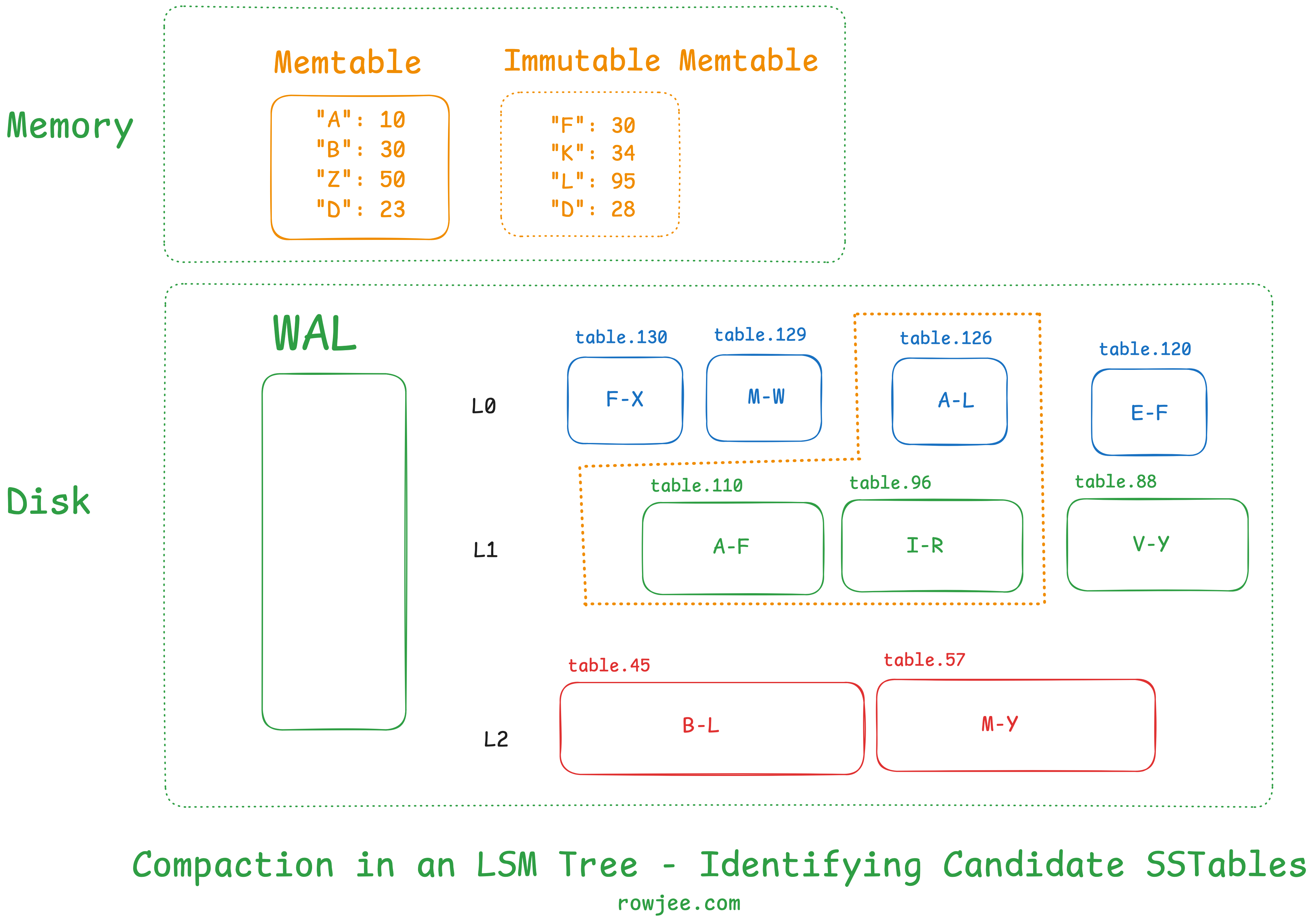
Now that we know what compaction is, let's explore how it happens in LSM Trees. This usually depends heavily on the implementation, but the general practice is that we pick a file from a level and merge it into files that have an overlapping key range in the next level. This is to maintain the invariant we spoke about in the previous part, where each level has only one file that a key can be in, which is why we need to have non-overlapping key ranges.

First, we identify the target SSTables that we need to compact. How we decide which sstables we want to compact also has massive performance implications. For now, we will just pick an overlapping key range.

Fundamentally, compaction is a merge sort on two very large sorted arrays of key-value pairs, where we maintain the hierarchy of sorting order as first by key, and then by creation time; then we simply discard all the values for a key except for the first one. This gives us an SSTable in memory!

Most LSM Trees usually use some sort of iterators to do this, as it is memory-efficient to page disk blocks in one by one, and because each table is sorted, we know that the iterator will move in only one direction. RocksDB for example has a MergingIterator² that helps them do this, with the examples provided.

Conversely, if we wish to iterate over two SSTables with a non-overlapping key range in the same level, we can simply "join" (read one after the other) the two SSTables. We accomplish this via a Join Iterator.

The final iterator construction looks something like this:

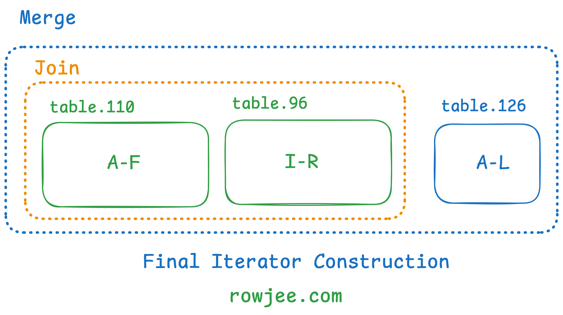
I won't cover the implementation details of the iterators now, but the output it gives us is similar to the hand-computed output we found at the end of our last example.

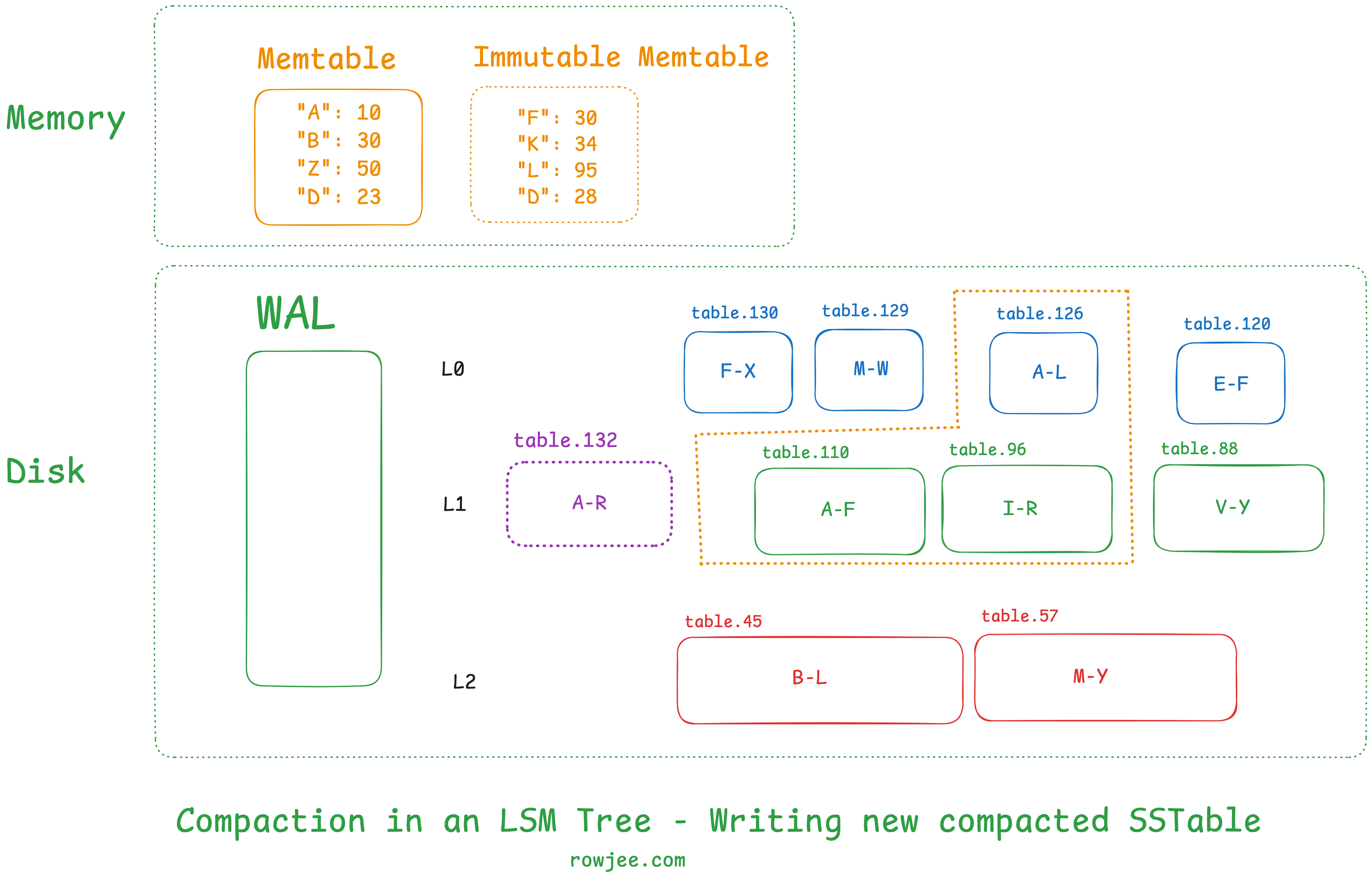
Once we've selected our candidate SSTables, we assemble the iterators, which materialize the output SSTable. As we read through the iterator, we write the new SSTable into the larger level of the levels we've chosen.

Then, we save the new state of the LSM Tree (level information, etc) in some kind of persistent state, such that the tree knows to look for this SSTable as a part of this level.

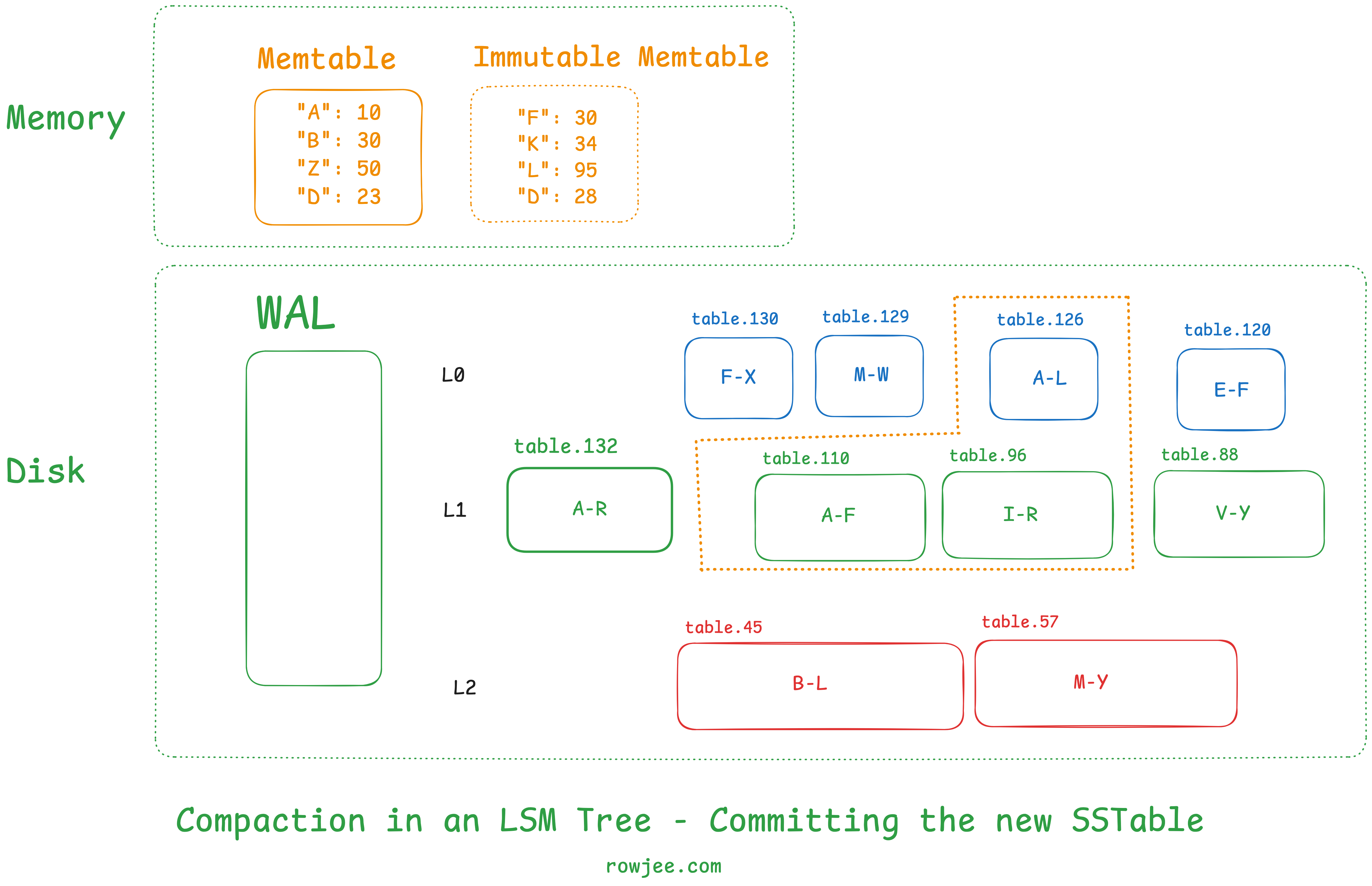
Lastly, we delete the old SSTables in the tree to reclaim our disk space.

As you can see, we've maintained the invariant that all levels of the table (except for level 0) have non-overlapping key ranges.

A good question to think about is: what do we do with tombstones during the compaction process?

Types of compaction

Now that we know that compaction also serves the process of maintaining not just data size but also the index by which we serve reads (the files, the levels, and the metadata for each level), there are multiple types of compaction strategies, each of which have different effects on lookup cost. There are multiple strategies present today, and this is an area of active research; A paper titled "Constructing and Analyzing the LSM Compaction Design Space"³ dives much deeper into this topic, and would be a good read for anyone trying to get a comprehensive view.

I won't be covering more compaction strategies in this post, but i'll probably expand upon this later.

Footnotes

1. https://smalldatum.blogspot.com/2015/11/read-write-space-amplification-pick-2_23.html ↩

2. https://github.com/facebook/rocksdb/wiki/Iterator-Implementation#mergingiterator ↩

3. https://vldb.org/pvldb/vol14/p2216-sarkar.pdf ↩