In this article, I'll be going through the paper "MapReduce: Simplified Data Processing on Large Clusters" by Jeffery Dean and Sanjay Ghemawat.
This paper deals with MapReduce, a way to perform large-scale computations with the fundamental operations (and functional primitives) map and reduce, in a distributed, parallelized manner.
If you're unfamiliar with the concepts here, I introduce the problem, and some basic primitives, in the background section - Keep reading for that! If you already know what these primitives are, and want to get to the paper directly, click here.
Table of Contents
- Background
- The Paper's Contributions
- Implementation
- Execution
- Metrics, Benchmarks and Performance
- MapReduce at Google
- Assumptions and limitations
- Conclusion
Background
To search the World Wide Web, one must first know what's on the web. To that end, one must generate a index - a data structure that holds both an item, and it's location.
In the same way the index of a book holds the name of the chapter and the page that chapter begins on, if one wishes to search the big ol' WWW by, say, a word, they'll need to maintain an index consisting of the item (the word being searched for) and its location (the URL of the page where the word is found).
Thus, creating an index of the WWW is the problem that Google faced in their early days. Way back then, the internet was (and mostly still is) a collection of HTML Documents maintaining links to each other by means of Hyperlinks (now URLs).
To generate an index, Google had to process as many parts of the web (as many documents) as they could, and perform said computations on it. However, this wasn't an easy problem at all - by around 1998, when Google launched, 512MB of RAM was a luxury, and there were already 2.4 Million websites on the internet 1. There were a lot of documents to process.
At the time, Engineers at Google had already solved this problem, by hand-rolling their own, case-specific implementations of a computing system for each task (indexing the web, running the PageRank Algorithm, and so on). They'd get hundreds or thousands of computers together on a network, get them to talk to each other, and co-ordinate these large tasks.
This was the only way these tasks would finish in a reasonable amount of time. However, these implementations ran into various issues, such as frequently failing disks, tasks that took too long to run, and so on.
Around this time, the authors of the paper noticed that most such compute-intensive tasks they ran at Google comprised of a series of map and reduce operations.
Map and Reduce are both primitives of Functional Programming, that allow you to use functions as arguments to another function.
Map
The map function takes in an array and a function, and it applies that function to every element of the array.
>>> def square(x):
...     return x * x
>>> a = [1, 2, 3, 4, 5]
>>> list(map(square, a))
[1, 4, 9, 16, 25]
Reduce
The reduce function takes an array and a function, and uses that function to combine the elements of the array.
>>> from functools import reduce
>>> def add(a, b):
...     return a + b
...
>>> a = [1, 2, 3, 4, 5]
>>> reduce(add, a)
15
Keep in mind that these map and reduce functions can be anything!
The Paper's Contributions
I see the paper having made two major contributions -
- Programs written as a series of Map and Reduce operations (and there are many that can be written this way) can be easily parallelized and distributed while maintaining an easy, simple interface
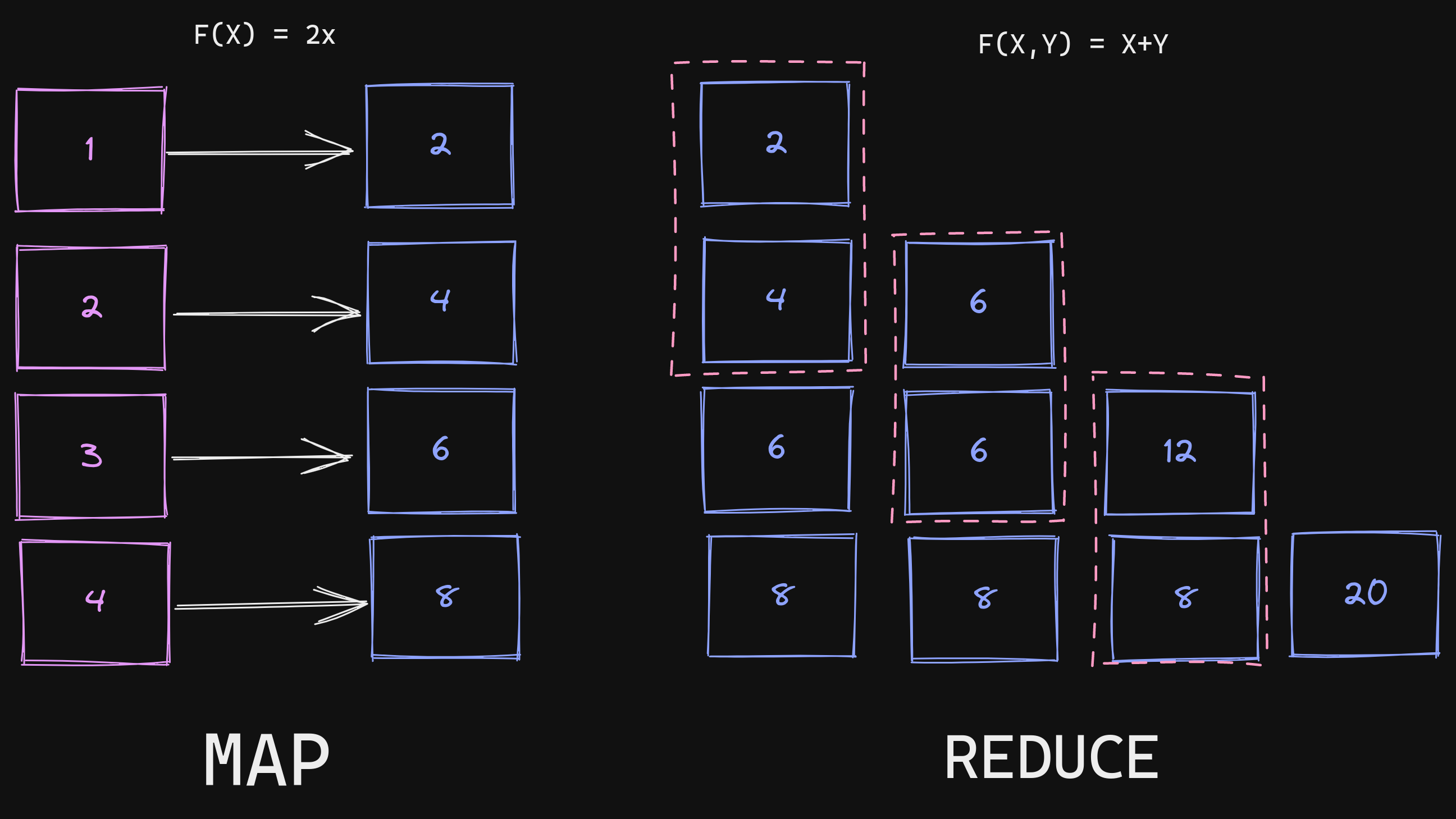 A simple example of a MapReduce program to find the sum of twice a list of numbers
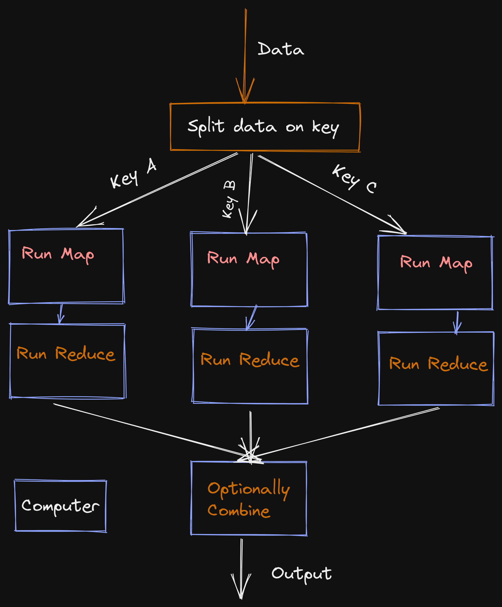 An example of how individual computers can handle map and reduce operations, enabling high parallelism and performance
Note that this paradigm consists of users only providing the functions that will be run on the map and reduce operations. They needn't worry about how or where it's implemented - they were inherently parallelizeable and could be distributed across multiple computers.
- A high-performance implementation of this interface on a large cluster of commodity computers
Google implemented a MapReduce system on a large cluster of commodity computers (~1000), which allowed them to complete indexing the internet in only seven passes of MapReduce.
The Programming Model
For the map function, the user provided a function that would take in some arguments (usually two, referred to as an "input pair"), and which emitted a series of intermediate key-value pairs.
The reduce function must then be written to accept a specific key, and a set of values for that key. It then reduces them to either form
- A smaller set of values, or
- One output value
From the paper, this can be summarized as the following -
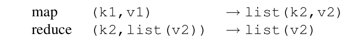 MapReduce functions described as types, taken from the paper
The map function takes in a key-value pair, and emits a list of key-value pairs. One can think of these keys emitted as "intermediate keys".
The reduce function takes in an intermediate key and a list of values for the same key, and emits a list of values (which can also have only one value).
The intermediate keys serve to help create a separation between different reduce jobs. Reduce Jobs for the Intermediate key "I" will only handle values coming which have been emitted with the Intermediate key "I".
Google's implementation uses some very clever tricks to make sure that intermediate key-value pairs for a key A emitted by the map job end up at the system running the reduce job for the same key. We'll explore this some more soon.
Some Programs in Google's MapReduce
Let's start off with the simplest example.
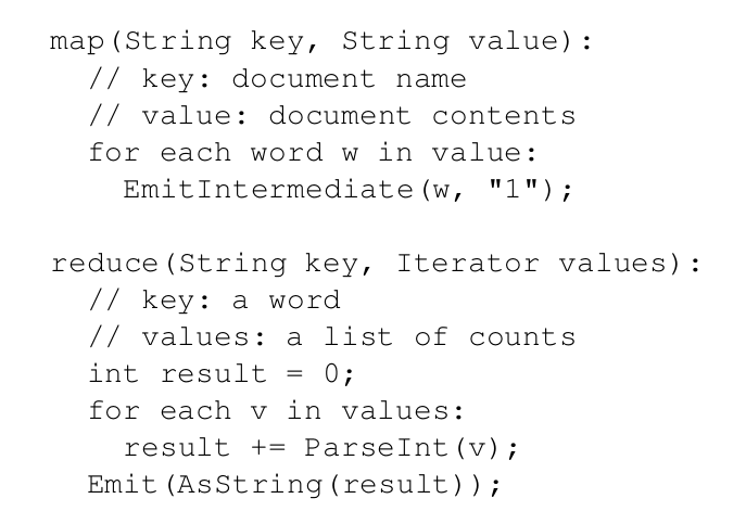 A MapReduce program to count the number of times each word occurs in a document or a string, taken from the paper
Here, emitIntermediate is a function used to emit an Intermediate key-value pair. emit is used to emit the final value after the reduce job completes.
Note that it's possible to perform many, many types of computation with this model. The paper mentions a few, one of which we'll take a look at here. Apart from the one here, the paper also mentions
- A Distributed Text Search
- URL Access Frequency Count
- Term-Vector per Host
- Inverted Index
- Distributed Sorting
Reverse Web-Link Graph with MapReduce
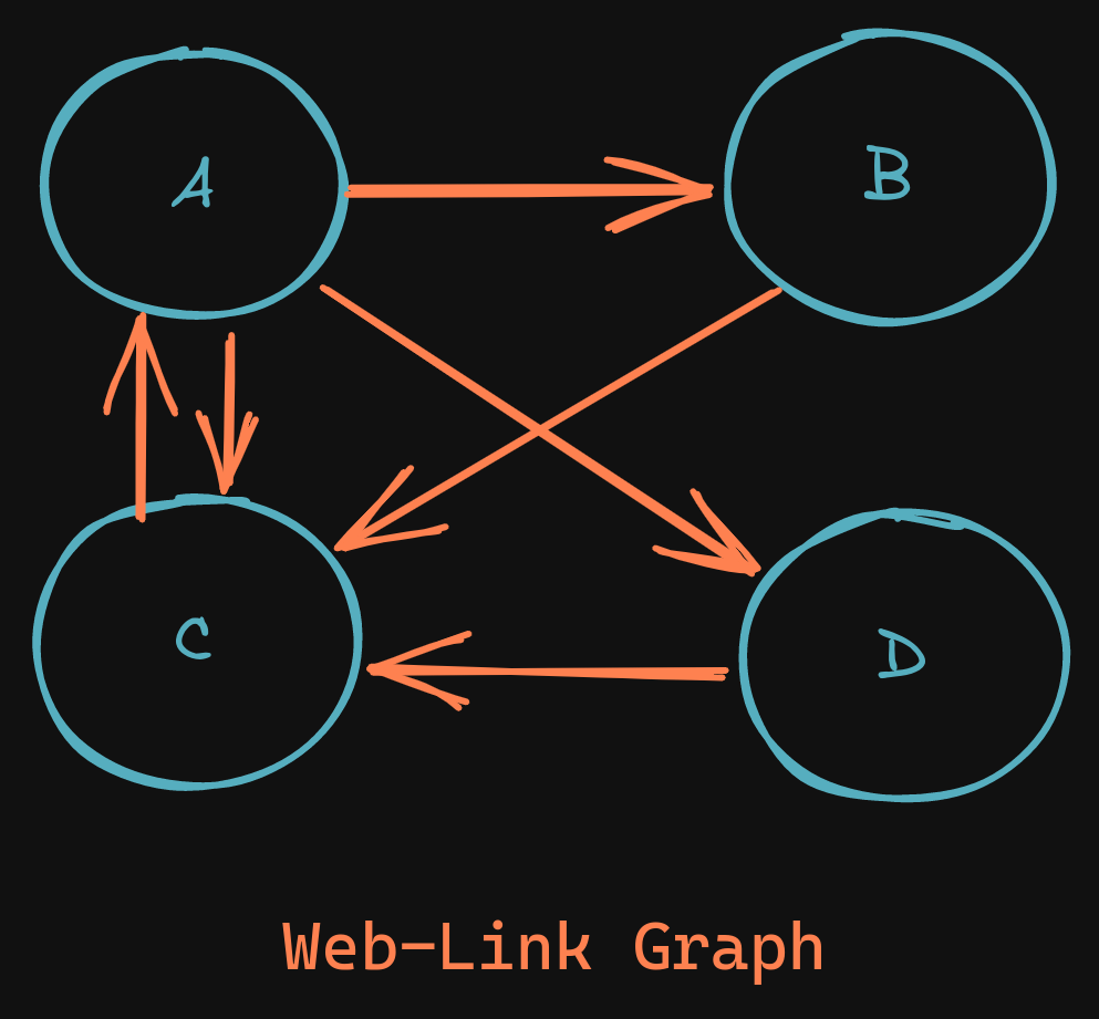 A simple example of four webpages, linking to each other
Let's say you want to find a list of pages (call them sources) that link to a specific page (the target) via a hyperlink.
This might be important, because you might want to rank how "important" a page is by seeing how many people link to it. Let's look at the page C.
Here's what our map function looks like -
def map(target, webpage):
  # check all the links in the page
  for link in webpage:
      # emitIntermediate(target, source)
      emitIntermediate(link, webpage.url)
Here are our intermediate values generated -
[(b, a), (d, a), (c, a), (c, b), (c, d), (a, c)]
Note that we're using the target link as our intermediate key.
Implementation Magic makes available to each reduce function the following -
[
(b, [a]),
(a, [c]),
(c, [a, b, d]),
(d, [a]),
]
Now, here's reduce -
def reduce(key, list):
    count = 0
    for link in list:
        count += 1
    emit(key, count)
Once reduce is called for all pages [a, b, c, d], we get -
[
(c, 3),
(a, 1),
(b, 1),
(c, 1)
]
This tells us that c is the most "important" page.
Implementation
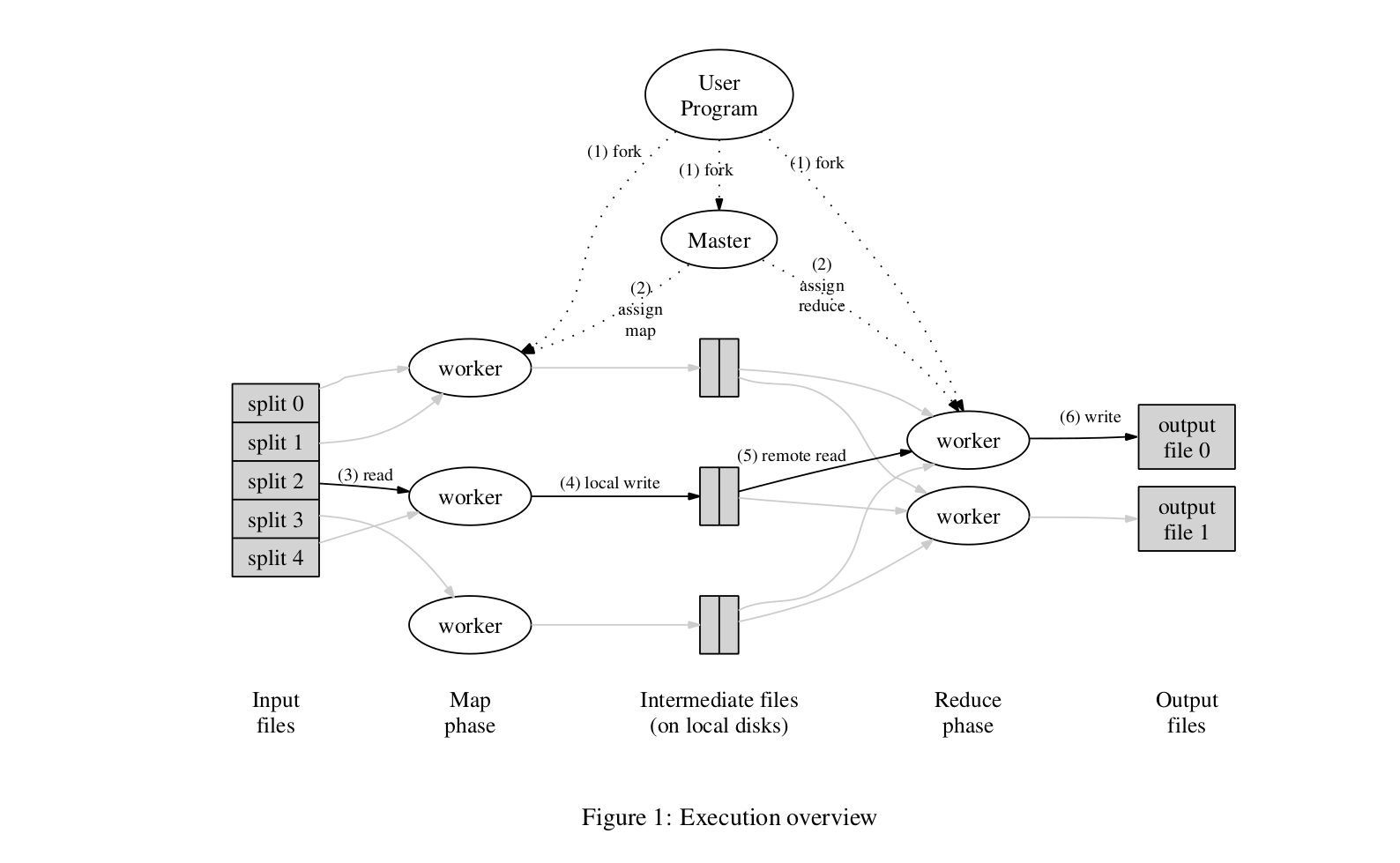 Google's implementation, as suggested in the paper
Now that we know how to implement some common programs in MapReduce, let's see how Google did it.
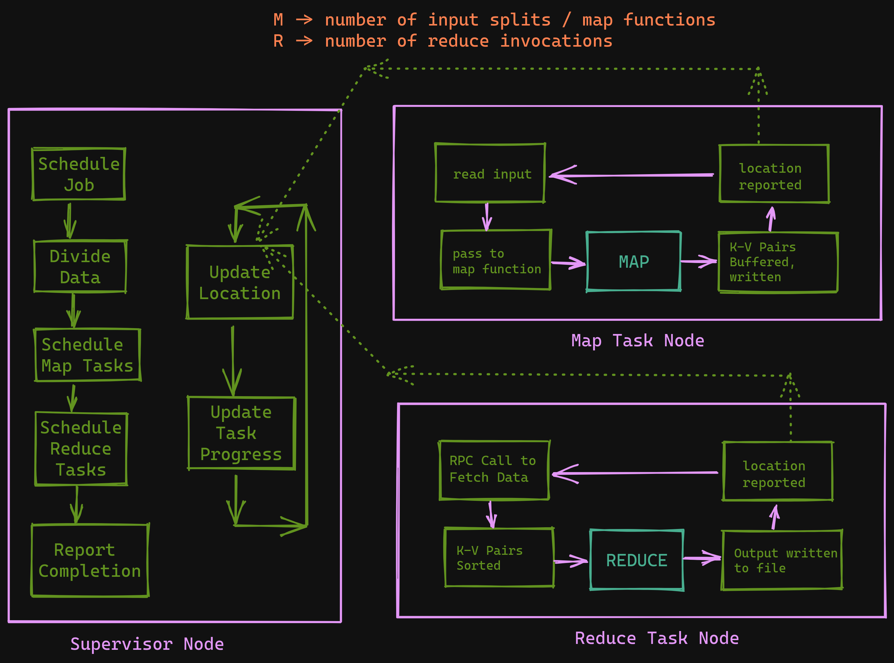
It all starts with a Master (we'll call this the Supervisor) process or worker node, which controls, schedules and orchestrates multiple MapReduce jobs on a cluster of commodity machines, each known as a worker node (we'll call these the Task nodes).
The task nodes can be threads, processes, or independent computers. For now, we'll only consider the last aspect.
Every task node is considered a generic task node, and isn't limited to being used only in the map or reduce phases of the entire process.
The supervisor node controls what job to schedule on which task node and when, so a node which ran map, if free, can also be used to run reduce.
The Scheduler also takes care of splitting data by key, or by size, to make it easier to transfer.
Execution
 Execution overview - MapReduce
-
The data to be processed is split into
Mpieces of 16Mb - 64Mb blocks. This block size can be controlled by the user. At this same time, the program is started on multiple machines. -
The Supervisor program is spawned, and it assigns work to all the Task Nodes. The Supervisor node also assigns idle nodes to different MapReduce Jobs.
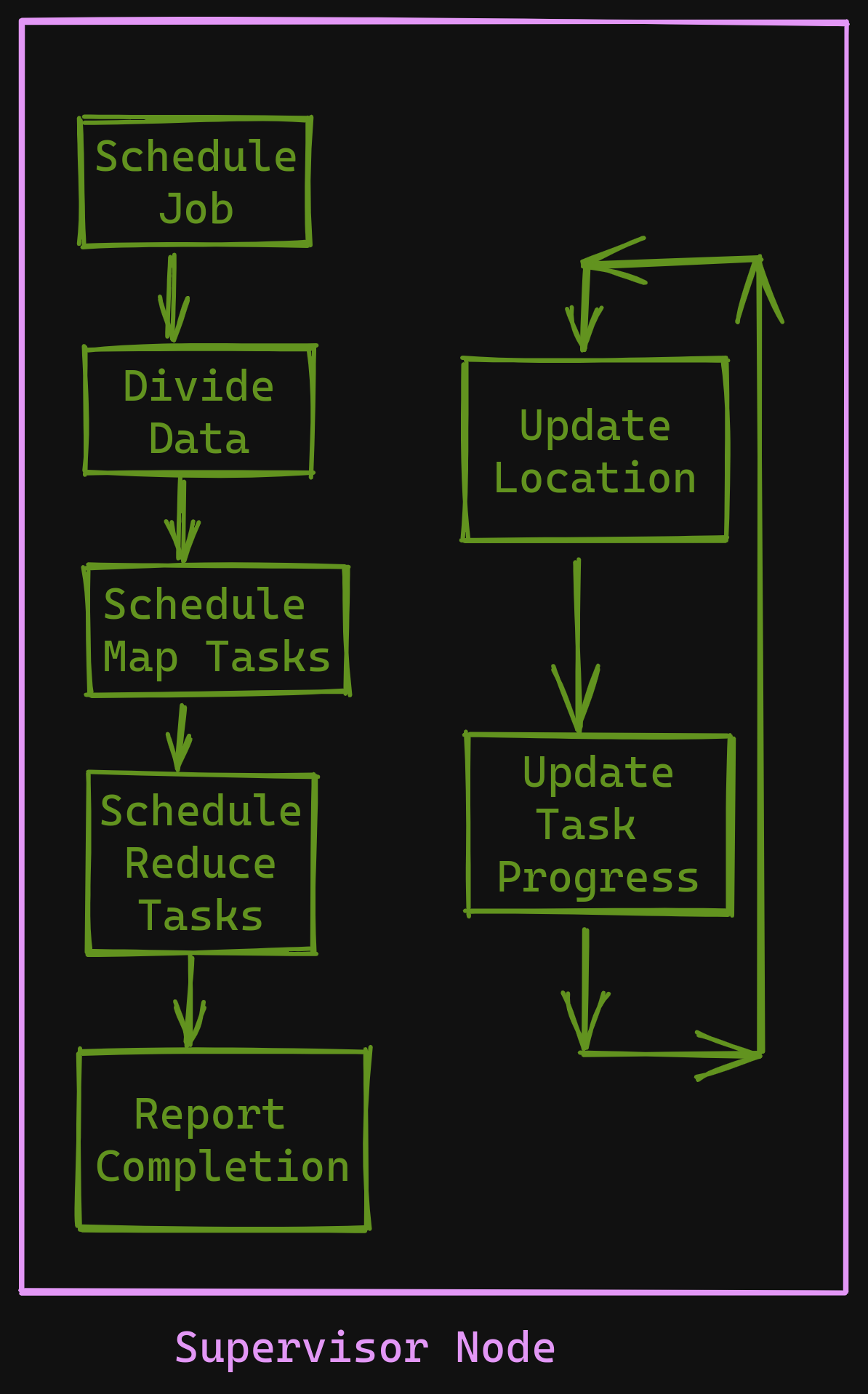 Execution Overview - Supervisor Node
- On the
mapside- Read the input assigned
- Parse the Key-Value pairs and pass them to the
mapfunction - Intermediate key-value pairs are buffered in-memory
- These buffered pairs are written to disk at regular intervals, and they're written partitioned by the key.
- The locations of these pairs are passed to the Supervisor node.
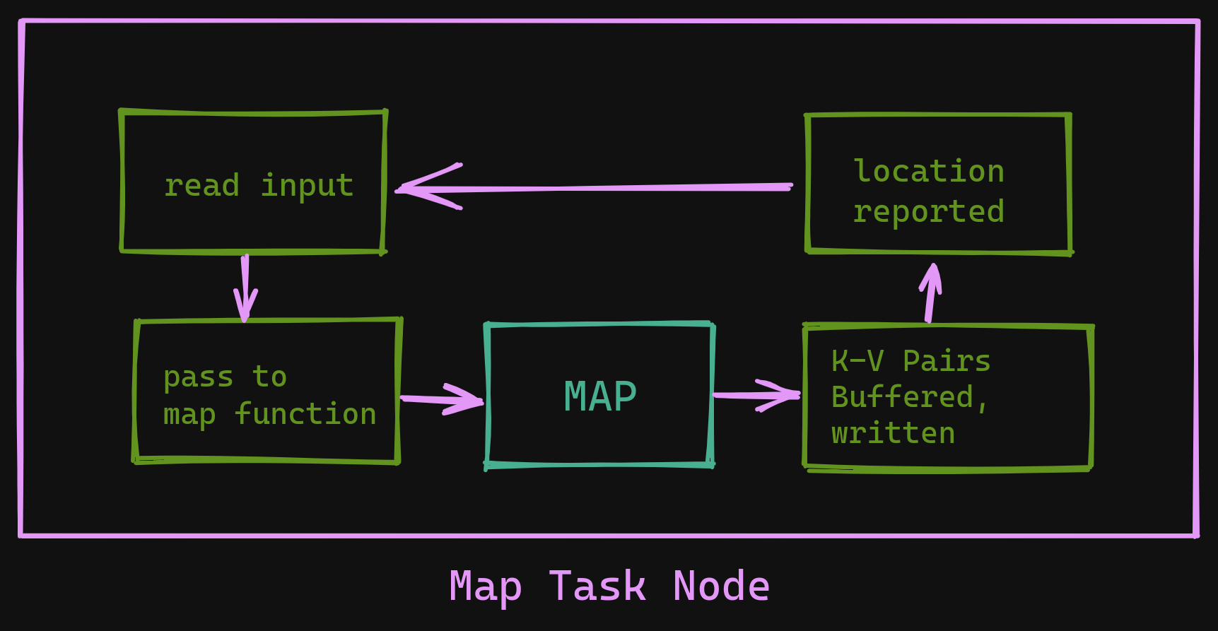 Execution Overview - Map Task Node
- On the
reduceside- When a
reducejob is scheduled, it uses a Remote Procedure Call to fetch the buffered pairs from themapworker. - Once all intermediate data has been obtained, the
reducetask node SORTS the key-value pairs to ensure the same pairs are grouped together. - The task node iterates over the data, passes the key-value pairs to the reduce function.
- The Output from this is appended to the final output file.
- When a
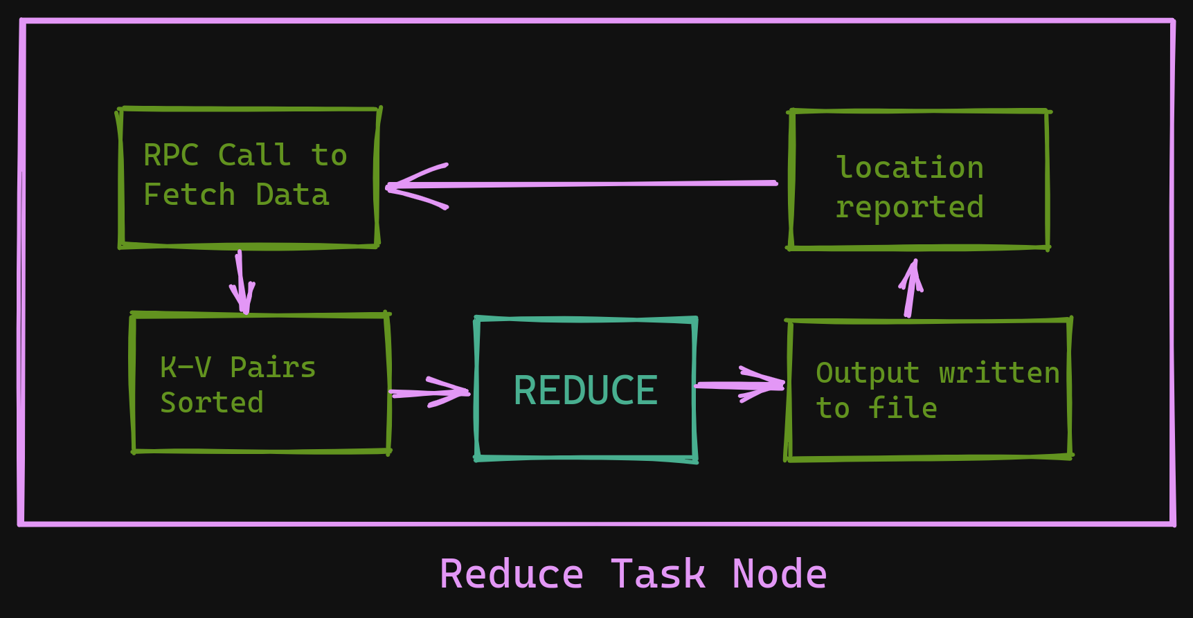 Execution Overview - Reduce Task Node
- The task is complete!
A (very cool) Note on Locality
One of Google's primary concerns was the reduction of network bandwidth being used, as it was a bottleneck. To prevent this from happening, Google implemented the Google File System (the GFS) - a distributed filesystem - to ensure that data was where it needed to be before it was required.
How the GFS works internally is perhaps the subject of another blog post itself, so we won't be concerning ourselves with that right now.
GFS (Google File System) handles moving files around, with a focus on ensuring that as much data is stored locally as possible. It also relies on replication - by dividing each file into 64MB Blocks, and ensuring that (typically) at least 3 copies of each block are available on different Task Nodes.
The coolest part is that the Supervisor Node is aware of this replication and locality effort, and attempts to schedule tasks on Task Nodes which already have the input files necessary to run the task. If one isn't available, it places the task on a machine close to (i.e. in the same network as) the replica. This way, bandwidth doesn't need to be wasted to move blocks back and forth.
A smaller note on Supervisor Data Structures
The supervisor node utilizies a number of data structures to keep track of all the tasks present in the cluster.
For every map and reduce task, it stores state (IDLE | INPROGRESS | COMPLETED) and the identity of task nodes.
For every completed map task, it stores the locations and sizes of the intermediate files produced. Updates happen as and when files are added or written to, and the same information is propagated to the reduce workers (this is only for INPROGRESS tasks)
Fault Tolerance
Such massive distributed systems can fail for multiple reasons. These are known as "Failure Modes", and there are many possible cases. The sheer scale of operation implies that failure is a regular event, not a special edge case.
If A Task Node Fails...
The Supervisor pings every Task Node periodically to ensure it's still alive. This is standard practice in most systems like this.
If a Task Node is dead (i.e. has not responded to the Supervisor after a threshold amount of time), all the tasks assigned (both completed and inprogress) to it get marked as IDLE and thus become eligible to be allocated to another node in the cluster.
Even the COMPLETED tasks are marked as IDLE as a Task Node stores its intermediate K-V pairs locally - if the node is inaccessible, then so are these intermediate K-V Pairs.
If The Supervisor Node Fails...
The Supervisor data structures written to disk, if a master fails, it's easy to restore it at that current state
Atomicity and Semantics in the presence of failures
The paper makes the following statement -
"When the user-supplied map and reduce operators are deterministic functions of their input values, our distributed implementation produces the same output as would have been produced by a non-faulting sequential execution of the entire program."
This is accomplished by using periodic, atomic writes of both the map and reduce outputs on their Task Nodes.
Since the writes are atomic, and the outputs are deterministic, even multiple runs of the same task will give the same output. Since it's atomic, there won't be any partial writes.
Dealing with Slower Machines by using Backup Tasks
Some nodes are stragglers - they become slow and hold up the scheduling queue, while completing one or a few of the LAST COUPLE OF REMAINING MapReduce tasks in a cluster. This slows down completion.
When an operation is close to completion, the Supervisor system schedules backup executions of the remaining INPROGRESS tasks, so at least one version will complete. This scheduling is tuned to increase the overall workload by only a few per cent.
Metrics, Benchmarks and Performance
The benchmarks for this cluster were considered mainly for two tasks -
- Sorting 1 TB of Data
- Searching 1 TB of Data
They were performed on a MapReduce cluster comprising roughly 1,800 computers, with 2x 2GHz Intel Xeon Processors, 4GB RAM, and 160GB IDE Disks per machine.
They find that Backup task handling proves to be crucial, absence of which proves to increase time by an average of 44%. The cluster is relatively resistant (only 5% delay) to machine failures, or process failures, at an 11.454% failure rate.
Sorting
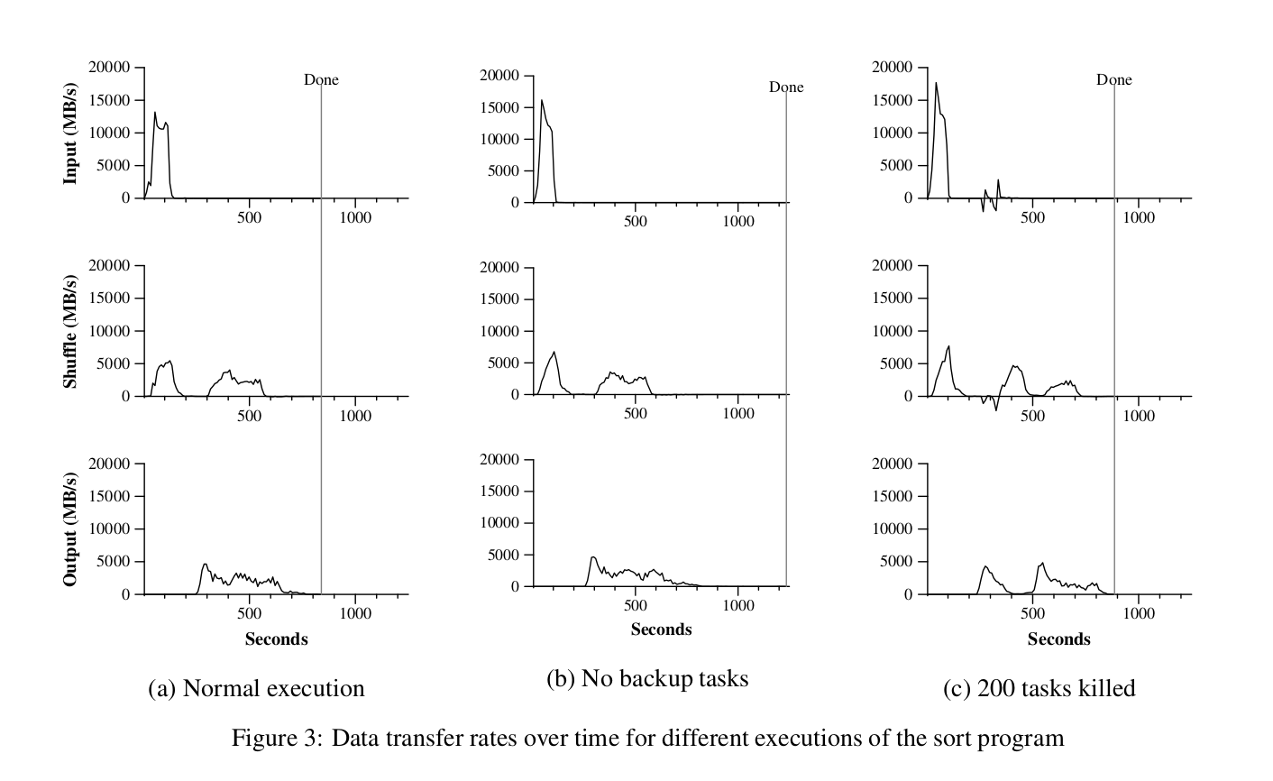
Data Transfer rate as a heuristic to estimate throughput of task completion. Notice how not having backup tasks makes a significant difference - Taken from the Paper
Each row in the above graph represents a different phase of the sorting task, where
- input - data read into the map jobs
- shuffle - buffered pairs from map jobs sent to reduce jobs and sorted
- output - reduce tasks complete and write to final output files
And each column corresponds to a different cluster configuration, being
- Normal Execution (with Backup Tasks)
- No Backup Tasks
- With 200 Tasks being killed off
This was modelled after the TeraSort benchmark. Since the reduce function sorts by keys, the Distributed Sort is fairly simple to implement in MapReduce.
Assuming a pre-existing knowledge of key distribution, Google's sorting implementation completed the sorting in 891 Seconds, as opposed to the current record, coming in at 1057 Seconds.
Searching
The implementation searched through 1 TB data in ~150 seconds, including around 60 seconds of startup time. Some delays and overheads were due to -
- Interactions with GFS
- getting the program to newly assigned machines
MapReduce at Google
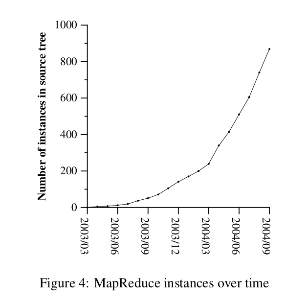 A graph showing the usage of MapReduce at Google
This was obviously a game-changer for Google, who began to use MapReduce not only for their production indexing system, but also for multiple other Google Services.
Their production indexing system crawled through 20TB of Data using MapReduce, with around Five to Ten passes of MapReduce for the entire indexing job. The same system went from around 3800 Lines of C++, to around 700 Lines when used with MapReduce.
Lastly, it allowed programmers who aren't distributed systems experts to take advantage of the infrastructure that Google has, as it abstracts away all the fault tolerance, parallelization, locality optimization and load-balancing details from the programmer. Since it focussed specifically on reducing network bandwidth usage, it allowed Google to deploy it at the scale we saw it run.
Assumptions and Limitations
- Assume functions being passed as Map and Reduce functions do not depend on Global State
- Assumes the Supervisor node can make scheduling decisions at scale - must make
O(M + R)scheduling decisions, and must keepO(M * R)state in memory. - Google's implementation assumes the task is restarted if the Supervisor Node fails
- No guarantee of similar performance in sorting benchmarks without prior knowledge of key distribution
Conclusion
This was my first ever paper review! If you liked it, do reach out to me to let me know what you think about it. I've got papers in mind that I want to cover, but if you find a paper you think is really cool, please don't hesitate to reach out!
As a paper, this one was super well-written, and I found my questions having been answered before I knew I had them. 10/10 recommended read.